How to get started with GRIB2 weather data and Python

Downloading the Data

The first step is downloading data from Spire Weather’s File API.

This tutorial expects the GRIB2 messages to contain NWP data from Spire’s Basic data bundle.

For information on using Spire Weather’s File API endpoints, please see the API documentation and FAQ.

The FAQ also contains detailed examples covering how to download multiple forecast files at once using cURL.

For the purposes of this tutorial, it is assumed that the GRIB2 data has already been successfully downloaded, download a global 7-day weather forecast sample here.

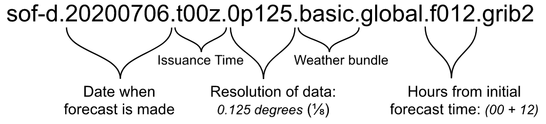
Understanding filenames

Files downloaded from Spire Weather’s API solutions all share the same file naming convention.

Just from looking at the filename, we can determine:

• the date and time that the forecast was issued
• the date and time that the forecasted data is valid for
• the horizontal resolution of the global forecast data
• the weather data variables that are included in the file (see the full list of Spire Weather’s commercial data bundles)

For more detailed information on the above, please refer to our FAQ.

Python Requirements

The following Python packages are required for this tutorial.

Although using conda is not strictly required, it is the officially recommended method for installing PyNIO (see link below).

Once a conda environment has been created and activated, the following commands can be run directly:

• conda install -c anaconda xarray

  • Details: http://xarray.pydata.org/
  • https://anaconda.org/anaconda/xarray

• conda install -c conda-forge pynio

  • Details: https://www.pyngl.ucar.edu/Nio.shtml
  • https://anaconda.org/conda-forge/pynio

If you’re having trouble with PyNIO, you can use cfgrib as the xarray engine instead: https://pypi.org/project/cfgrib/

• conda install -c anaconda pandas

  • Details: https://pandas.pydata.org/
  • https://anaconda.org/anaconda/panda

Inspecting the Data

After downloading the data and setting up a Python environment with the required packages, the next step is inspecting the data contents in order to determine which weather variables are available to access. Data inspection can be done purely with PyNIO, but in this tutorial we will instead use PyNIO as the engine for xarray and load the data into an xarray dataset for transformation. Note that an explicit import of PyNIO is not required, so long as it’s installed properly in the active Python environment.

First, import the xarray package:

import xarray as xr

Next, open the GRIB2 data with xarray using PyNIO as its engine (note that the GRIB2 data should be from Spire’s Basic data bundle):

ds = xr.open_dataset("path_to_basic_file.grib2", engine="pynio")

Finally, for each of the variables, print the lookup key, human-readable name, and units of measurement:

for v in ds:
    print("{}, {}, {}".format(v, ds[v].attrs["long_name"], ds[v].attrs["units"]))

The output of the above should look something like this, giving a clear overview of the available data fields:

TMP_P0_L103_GLL0, Temperature, K
DPT_P0_L103_GLL0, Dew point temperature, K
RH_P0_L103_GLL0, Relative humidity, %
UGRD_P0_L103_GLL0, U-component of wind, m s-1
VGRD_P0_L103_GLL0, V-component of wind, m s-1
GUST_P0_L1_GLL0, Wind speed (gust), m s-1
PRMSL_P0_L101_GLL0, Pressure reduced to MSL, Pa
APCP_P8_L1_GLL0_acc, Total precipitation, kg m-2

For more details, the full metadata of each variable can be inspected as well: print(ds["TMP_P0_L103_GLL0"])

Processing the Data

Now that we know precisely which weather variables are included in the GRIB2 data, we can start processing our xarray dataset.

Filtering the xarray data to a specific variable

With xarray, filtering the dataset’s contents to a single variable of interest is very straightforward:

ds = ds.get("TMP_P0_L103_GLL0")

Selecting multiple variables is also possible by using an array of strings as the input: ds = ds.get([var1, var2])

It’s recommended to perform this step before converting the xarray dataset into a pandas DataFrame (rather than filtering the DataFrame later), since it minimizes the size of the data being converted and therefore reduces the overall runtime.

Converting the xarray data into a pandas.DataFrame

To convert the filtered xarray dataset into a pandas DataFrame, simply run the following:

df = ds.to_dataframe()

Cropping the pandas.DataFrame to a geospatial bounding box

After the filtered data is converted into a pandas DataFrame, we can crop it to a specific area of interest.

The first step in this process is unpacking the latitude and longitude values from the DataFrame’s index, which can be accessed through the index names of lat_0 and lon_0:

latitudes = df.index.get_level_values("lat_0")
longitudes = df.index.get_level_values("lon_0")

Although latitude values are already in the standard range of -90 degress to +90 degrees, longitude values are in the range of 0 to +360.

To make the data easier to work with, we convert longitude values into the standard range of -180 degrees to +180 degrees:

map_function = lambda lon: (lon - 360) if (lon > 180) else lon
remapped_longitudes = longitudes.map(map_function)

With latitude and longitude data now in the desired value ranges, we can store them as new columns in our existing DataFrame:

df["longitude"] = remapped_longitudes
df["latitude"] = latitudes

The next step in the process is defining our geospatial bounding box, which we do by specifying the minimum and maximum coordinate values:

min_lat = 10.2
max_lat = 48.9
min_lon = -80
max_lon = -8.3

Then, we use the bounding box values to construct the DataFrame filter expressions:

lat_filter = (df["latitude"] >= min_lat) & (df["latitude"] <= max_lat)
lon_filter = (df["longitude"] >= min_lon) & (df["longitude"] <= max_lon)

Finally, we apply the filters to our existing DataFrame:

df = df.loc[lat_filter & lon_filter]

The resulting DataFrame has been cropped to the bounds of the box that we specified above.

Parsing the forecast time from the filename

Each individual file contains global weather forecast data for the same point in time.

Using our knowledge from the Understanding Filenames section of this tutorial, and assuming that the filename argument is in the expected format, we can write a function to parse the valid forecast time from the filename:

from datetime import datetime, timedelta

def parse_datetime_from_filename(filename):
    parts = filename.split(".")
    # Parse the forecast date from the filename
    date = parts[1]
    forecast_date = datetime.strptime(date, "%Y%m%d")
    # Strip `t` and `z` to parse the forecast issuance time (an integer representing the hour in UTC)
    issuance_time = parts[2]
    issuance_time = int(issuance_time[1:3])
    # Strip `f` to parse the forecast lead time (an integer representing the number of hours since the forecast issuance)
    lead_time = parts[-2]
    lead_time = int(lead_time[1:])
    # Combine the forecast issuance and lead times to get the valid time for this file
    hours = issuance_time + lead_time
    forecast_time = forecast_date + timedelta(hours=hours)
    # Return the datetime as a string to store it in the DataFrame
    return str(forecast_time)

Then, we can create a new DataFrame column for time which stores this value as a string in every row:

timestamp = parse_datetime_from_filename(filename)
df["time"] = timestamp

Although it may seem unnecessary to store the same exact timestamp value in every row, this is an important step if we want to eventually concatenate our DataFrame with forecast data for other times (demonstrated below in Processing Multiple Data Files).

Saving the data to a CSV output file

Perform a final filter on our DataFrame to select only the columns that we want in our output, where variable is a string like "TMP_P0_L103_GLL0" :

df = df.loc[:, ["latitude", "longitude", "time", variable]]

Save the processed DataFrame to an output CSV file:

df.to_csv("output_data.csv", index=False)

Setting the index=False parameter ensures that the DataFrame index columns are not included in the output. This way, we exclude the lat_0 and lon_0 values and are left with just the latitude and remapped longitude columns.

Please note that converting from GRIB2 to CSV can result in very large file sizes, especially if the data is not significantly cropped or filtered.

Processing Multiple Data Files

It is often desirable to process multiple data files at once, in order to combine the results into a single unified CSV output file.

For example, let’s say that we have just used the Spire Weather API to download a full forecast’s worth of GRIB2 data into a local directory called forecast_data/. We can then read those filenames into a list and sort them alphabetically for good measure:

import glob

filenames = glob.glob("forecast_data/*.grib2")
filenames = sorted(filenames)

From here, we can iterate through the filenames and pass each one into a function that performs the steps outlined in the Processing the Data section of this tutorial.

Once all of our final DataFrames are ready, we can use pandas to concatenate them together like so (where final_dataframes is a list of DataFrames):

import pandas as pd

output_df = pd.DataFrame()

for df in final_dataframes:
    output_df = pd.concat([output_df, df])

We end up with a combined DataFrame called output_df which we can save to an output CSV file like we did before:

output_df.to_csv("combined_output_data.csv", index=False)

Complete Code

Below is an operational Python script which uses the techniques described in this tutorial and also includes explanatory in-line comments.

The script takes three arguments:

1. The weather data variable of interest

2. The local directory where the GRIB2 data is stored

3. The geospatial bounding box for cropping the data

   • Specified as a list of coordinate values separated by spaces:
     min_latitude max_latitude min_longitude max_longitude 

For example, the script can be run like this:

python script.py --variable TMP_P0_L103_GLL0 --source-data grib_directory/ --bbox 10.2 48.9 -80 -8.3

Here is the complete code:

from datetime import datetime, timedelta
import xarray as xr
import pandas as pd
import argparse
import glob
import sys
import os


def parse_datetime_from_filename(filename):
    """
    Assuming that the filename matches Spire's naming convention,
    this function will parse the valid forecast time from the filename.
    Example filename: `sof-d.20200401.t00z.0p125.basic.global.f006.grib2`
    """
    parts = filename.split(".")
    # Parse the forecast date from the filename
    date = parts[1]
    forecast_date = datetime.strptime(date, "%Y%M%d")
    # Strip `t` and `z` to parse the forecast issuance time (an integer representing the hour in UTC)
    issuance_time = parts[2]
    issuance_time = int(issuance_time[1:3])
    # Strip `f` to parse the forecast lead time (an integer representing the number of hours since the forecast issuance)
    lead_time = parts[-2]
    lead_time = int(lead_time[1:])
    # Combine the forecast issuance and lead times to get the valid time for this file
    hours = issuance_time + lead_time
    forecast_time = forecast_date + timedelta(hours=hours)
    # Return the datetime as a string to store it in the DataFrame
    return str(forecast_time)


def crop_dataframe_to_bbox(df, bbox):
    """
    Perform a geospatial filter on the DataFrame
    based on the specified bounding box
    """
    # Get longitude and latitude values from the DataFrame index
    longitudes = df.index.get_level_values("lon_0")
    latitudes = df.index.get_level_values("lat_0")
    # Map longitude range from (0 to 360) into (-180 to 180)
    map_function = lambda lon: (lon - 360) if (lon > 180) else lon
    remapped_longitudes = longitudes.map(map_function)
    # Create new longitude and latitude columns in the DataFrame
    df["longitude"] = remapped_longitudes
    df["latitude"] = latitudes
    # Unpack the bounding box values
    min_lat = float(bbox[0])
    max_lat = float(bbox[1])
    min_lon = float(bbox[2])
    max_lon = float(bbox[3])
    # Construct the DataFrame filters
    lat_filter = (df["latitude"] >= min_lat) & (df["latitude"] <= max_lat) lon_filter = (df["longitude"] >= min_lon) & (df["longitude"] <= max_lon)
    # Apply filters to the DataFrame
    df = df.loc[lat_filter & lon_filter]
    return df


def process_data(filepath, variable, bbox):
    """
    Load and process the GRIB2 data
    """
    # Load the files with GRIB2 data into an xarray dataset
    ds = xr.open_dataset(filepath, engine="pynio")
    # Retrieve only the desired values to reduce the volume of data,
    # otherwise converting to a DataFrame will take a long time.
    # To get more than 1 variable, use a list: `ds.get([var1, var2])`
    ds = ds.get(variable)
    # Convert the xarray dataset to a DataFrame
    df = ds.to_dataframe()
    # Perform an initial coarse filter on the global DataFrame
    df = crop_dataframe_to_bbox(df, bbox)
    # Parse the filename from the full filepath string
    filename = filepath.split("/")[1]
    # Convert the filename to a datetime string
    timestamp = parse_datetime_from_filename(filename)
    # Store the forecast time in a new DataFrame column
    df["time"] = timestamp
    # Trim the data to just the lat, lon, time, and weather variable columns
    df = df.loc[:, ["latitude", "longitude", "time", variable]]
    return df


if __name__ == "__main__":
    parser = argparse.ArgumentParser(description="Extract weather data within a region")
    parser.add_argument(
        "--variable",
        type=str,
        default="TMP_P0_L103_GLL0",  # This temperature variable is in the Basic data bundle
        help="The name of the weather data variable to extract",
    )
    parser.add_argument(
        "--source-data",
        type=str,
        help="The name of the directory containing properly formatted Spire GRIB2 data",
        required=True,
    )
    parser.add_argument(
        "--bbox",
        nargs="+",
        default=[36, 42, -10, -5],  # min_lat max_lat min_lon max_lon
        help="The bounding box used to crop the data, specified as minimum/maximum latitudes and longitudes",
    )
    # Parse the input arguments
    args = parser.parse_args()
    # Perform a simple check on the bounding box before proceeding
    if len(args.bbox) != 4:
        sys.exit(
            "The `bbox` argument must contain four values: `minlat maxlat minlon maxlon`"
        )
    # Read all data files in the specified directory
    filepath = os.path.join(args.source_data, "*.grib2")
    filenames = glob.glob(filepath)
    # Sort the filenames alphabetically
    filenames = sorted(filenames)
    # Initialize the output DataFrame
    output_df = pd.DataFrame()
    # For each file, process the data into a DataFrame
    # and concatenate all of the DataFrames together
    for file in filenames:
        print("Processing ", file)
        data = process_data(file, args.variable, args.bbox)
        if data is not None:
            output_df = pd.concat([output_df, data])
    # Save the final DataFrame to a CSV file
    # and do not include the index values (`lat_0` and `lon_0`)
    # since we created new `latitude` and `longitude` columns
    output_df.to_csv("output_data.csv", index=False)

Final Notes

Using the CSV data output from our final script, we can now easily visualize the processed data in a free tool such as kepler.gl. We can also set thresholds for alerts, generate statistics, or fuse with other datasets.

The storm tracking visualizations included here – originally featured in a Spire data story – were all created with Kepler using the techniques covered in this tutorial. Other visualizations in the data story are created with Spire’s Web Map Service (WMS) API which you can read more about here.

For additional code samples, check out Spire Weather’s public GitHub repository.