How to process GRIB2 weather data for maritime applications (Shapefile)

Downloading the Data

The first step is downloading data from Spire Weather’s File API.

This tutorial expects the GRIB2 messages to contain NWP data from Spire’s Maritime data bundle.

For information on using Spire Weather’s File API endpoints, please see the API documentation and FAQ.

The FAQ also contains detailed examples covering how to download multiple forecast files at once using cURL.

For the purposes of this tutorial, it is assumed that the GRIB2 data has already been successfully downloaded, if not you can get a global weather forecast sample here.

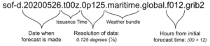
Understanding filenames

Files downloaded from Spire Weather’s API solutions all share the same file naming convention.

Just from looking at the filename, we can determine:

• the date and time that the forecast was issued
• the date and time that the forecasted data is valid for
• the horizontal resolution of the global forecast data
• the weather data variables that are included in the file (see the full list of Spire Weather’s commercial data bundles)

For more detailed information on the above, please refer to our FAQ.

Python Requirements

The following Python packages are required for this tutorial.

Although using conda is not strictly required, it is the officially recommended method for installing PyNIO (see link below).

Once a conda environment has been created and activated, the following commands can be run directly:

• conda install -c anaconda xarray

  • Details: http://xarray.pydata.org/
  • https://anaconda.org/anaconda/xarray

• conda install -c conda-forge pynio

  • Details: https://www.pyngl.ucar.edu/Nio.shtml
  • https://anaconda.org/conda-forge/pynio

If you’re having trouble with PyNIO, you can use cfgrib as the xarray engine instead: https://pypi.org/project/cfgrib/

• conda install -c anaconda pandas

  • Details: https://pandas.pydata.org/
  • https://anaconda.org/anaconda/pandas

• conda install -c conda-forge gdal

  • Details: https://gdal.org/
  • https://anaconda.org/conda-forge/gdal

Inspecting the Data

After downloading the data and setting up a Python environment with the required packages, the next step is inspecting the data contents in order to determine which weather variables are available to access. Data inspection can be done purely with PyNIO, but in this tutorial we will instead use PyNIO as the engine for xarray and load the data into an xarray dataset for transformation. Note that an explicit import of PyNIO is not required, so long as it’s installed properly in the active Python environment.

First, import the xarray package:

import xarray as xr

Next, open the GRIB2 data with xarray using PyNIO as its engine (note that the GRIB2 data should be from Spire’s Maritime data bundle):

ds = xr.open_dataset("path_to_maritime_file.grib2", engine="pynio")

Finally, for each of the variables, print the lookup key, human-readable name, and units of measurement:

for v in ds:
    print("{}, {}, {}".format(v, ds[v].attrs["long_name"], ds[v].attrs["units"]))

The output of the above should look something like this, giving a clear overview of the available data fields:

HTSGW_P0_L101_GLL0, Significant height of combined wind waves and swell, m
WWSDIR_P0_L101_GLL0, Direction of combined wind waves and swell, degree true
MWSPER_P0_L101_GLL0, Mean period of combined wind waves and swell, s
UOGRD_P0_L1_GLL0, U-component of current, m s-1
VOGRD_P0_L1_GLL0, V-component of current, m s-1
WTMP_P0_L1_GLL0, Water temperature, K

For more details, the full metadata of each variable can be inspected as well: print(ds["HTSGW_P0_L101_GLL0"])

Processing the Data

Now that we know which weather variables are included in the GRIB2 data, we can start processing our xarray dataset.

Filtering the xarray data to a specific variable

With xarray, filtering the dataset’s contents to a single variable of interest is very straightforward:

ds = ds.get("HTSGW_P0_L101_GLL0")

Selecting multiple variables is also possible by using an array of strings as the input: ds = ds.get([var1, var2])

It’s recommended to perform this step before converting the xarray dataset into a pandas DataFrame (rather than filtering the DataFrame later), since it minimizes the size of the data being converted and therefore reduces the overall runtime.

Converting the xarray data into a pandas.DataFrame

To convert the filtered xarray dataset into a pandas DataFrame, simply run the following:

df = ds.to_dataframe()

Loading an Esri Shapefile with the GDAL Python package

Although the package we installed with conda was named gdal, we import it into Python as osgeo. This is an abbreviation of the Open Source Geospatial Foundation, which GDAL/OGR (a Free and Open Source Software) is licensed through.

from osgeo.ogr import GetDriverByName
driver = GetDriverByName("ESRI Shapefile")

The Shapefile format, originally developed by Esri, is a common standard in the world of geographic information systems. It defines the geometry and attributes of geographically referenced features in three or more files with specific file extensions. The three mandatory file extensions are .shp, .shx, and .dbf — and all of these related component files are expected to be stored in the same file directory. Many pre-existing Shapefiles can be downloaded for free online (e.g. national borders, exclusive economic zones, etc.) and custom shapes can also be created in a variety of free software tools. In this example we use the EEZ of Australia as our complex polygon, but this could just as easily be any other geographical area.

When opening a Shapefile with GDAL, we only need to point to the file with the .shp extension. However, it is required that the other component files exist in the same directory. If we are opening a file called eez.shp, there should at least be files named eez.shx and eez.dbf in the same directory as well.

import os
filename = os.path.join("shpfile/eez.shp")

Once we have defined the driver and the path to our Shapefile polygon, we can load it into our script like this:

shpfile = driver.Open(filename)
area = shpfile.GetLayer()

Getting the bounding box that contains a Shapefile area

Eventually we will crop the data to the precise area defined by the Shapefile, but this is a computationally expensive process so it’s best to limit the data size first. In theory we could skip the step of cropping to a simple box altogether, but in practice it’s worth doing so to reduce the overall runtime.

GDAL makes it easy to calculate the coarse bounding box that contains a complex Shapefile area:

bbox = area.GetExtent()

Coordinate values can then be accessed individually from the resulting array:

min_lon = bbox[0]
max_lon = bbox[1]
min_lat = bbox[2]
max_lat = bbox[3]

The order of geospatial coordinates is a common source of confusion, so take care to note that GDAL’s GetExtent function returns an array where the longitude values come before the latitude values.

Cropping the pandas.DataFrame to a geospatial bounding box

Now that the filtered data is converted into a pandas DataFrame and we have the bounds containing our area of interest, we can crop the data to a simple box.

The first step in this process is unpacking the latitude and longitude values from the DataFrame’s index, which can be accessed through the index names of lat_0 and lon_0:

latitudes = df.index.get_level_values("lat_0")
longitudes = df.index.get_level_values("lon_0")

Although latitude values are already in the standard range of -90 degress to +90 degrees, longitude values are in the range of 0 to +360.

To make the data easier to work with, we convert longitude values into the standard range of -180 degrees to +180 degrees:

map_function = lambda lon: (lon - 360) if (lon > 180) else lon
remapped_longitudes = longitudes.map(map_function)

With latitude and longitude data now in the desired value ranges, we can store them as new columns in our existing DataFrame:

df["longitude"] = remapped_longitudes
df["latitude"] = latitudes

Then, we use the bounding box values from the previous section (the components of the bbox array) to construct the DataFrame filter expressions:

lat_filter = (df["latitude"] >= min_lat) & (df["latitude"] <= max_lat)
lon_filter = (df["longitude"] >= min_lon) & (df["longitude"] <= max_lon)

Finally, we apply the filters to our existing DataFrame:

df = df.loc[lat_filter & lon_filter]

The resulting DataFrame has been cropped to the bounds of the box that contains the complex Shapefile area.

Cropping the pandas.DataFrame to the precise bounds of a Shapefile area

In order to crop the DataFrame to the precise bounds of the complex Shapefile area, we will need to check every coordinate pair in our data. Similar to the previous section where we remapped every longitude value, we will perform this action with a map expression.

To pass each coordinate pair into the map function, we create a new DataFrame column called point where each value is a tuple containing both latitude and longitude:

df["point"] = list(zip(df["latitude"], df["longitude"]))

We can then pass each coordinate pair tuple value into the map function, along with the previously loaded Shapefile area, and process them in a function called check_point_in_area which we will define below. The check_point_in_area function will return either True or False to indicate whether the provided coordinate pair is inside of the area or not. As a result, we will end up with a new DataFrame column of boolean values called inArea:

map_function = lambda latlon: check_point_in_area(latlon, area)
df["inArea"] = df["point"].map(map_function)

Once the inArea column is populated, we perform a simple filter to remove rows where the inArea value is False. This effectively removes data for all point locations that are not within the Shapefile’s area:

df = df.loc[(df[“inArea”] == True)]

Of course, the success of the above is dependent upon the logic inside of the check_point_in_area function, which we have not yet implemented. Since the Shapefile area was loaded with GDAL, we can leverage a GDAL geometry method called Contains to quickly check if the area contains a specific point. In order to do this,  the coordinate pair must first be converted into a wkbPoint geometry in GDAL:

from osgeo.ogr import Geometry, wkbPoint

ogr_point = Geometry(wkbPoint)
ogr_point.AddPoint(longitude, latitude)

All Shapefiles are composed of one or more feature, so to ensure our code is robust we will need to check each component feature individually. Features can be retrieved by their numerical index with area.GetFeature(i), and the total number of features can be retrieved with area.GetFeatureCount(). Using these two functions with the Contains method mentioned above, we can iterate through each feature and check if it contains the point geometry:

for i in range(area.GetFeatureCount()):
    feature = area.GetFeature(i)
    if feature.geometry().Contains(OGR_POINT):
        point_in_area = True

Putting the pieces together, here is what we get for our final check_point_in_area function:

def check_point_in_area(latlon, area):
    # Initialize the boolean
    point_in_area = False
    # Parse coordinates and convert to floats
    lat = float(latlon[0])
    lon = float(latlon[1])
    # Set the point geometry
    OGR_POINT.AddPoint(lon, lat)
    # Check if the point is in any of the shapefile's features
    for i in range(area.GetFeatureCount()):
        feature = area.GetFeature(i)
        if feature.geometry().Contains(OGR_POINT):
            # This point is within a feature
            point_in_area = True
            # Break out of the loop, since there's no need
            # to check the remaining features now
            break
    # Return flag indicating whether point is in the area
    return point_in_area

As you can see, the only variable returned by the check_point_in_area function is a boolean value indicating whether the specified point is in the area or not. These boolean values then populate the new inArea DataFrame column. This allows us to apply the filter from above and end up with the precisely cropped data we want:

df = df.loc[(df["inArea"] == True)]

Parsing the forecast time from the filename

Each individual file contains global weather forecast data for the same point in time.

Using our knowledge from the Understanding Filenames section of this tutorial, and assuming that the filename argument is in the expected format, we can write a function to parse the valid forecast time from the filename:

from datetime import datetime, timedelta

def parse_datetime_from_filename(filename):
    parts = filename.split(".")
    # Parse the forecast date from the filename
    date = parts[1]
    forecast_date = datetime.strptime(date, "%Y%m%d")
    # Strip `t` and `z` to parse the forecast issuance time (an integer representing the hour in UTC)
    issuance_time = parts[2]
    issuance_time = int(issuance_time[1:3])
    # Strip `f` to parse the forecast lead time (an integer representing the number of hours since the forecast issuance)
    lead_time = parts[-2]
    lead_time = int(lead_time[1:])
    # Combine the forecast issuance and lead times to get the valid time for this file
    hours = issuance_time + lead_time
    forecast_time = forecast_date + timedelta(hours=hours)
    # Return the datetime as a string to store it in the DataFrame
    return str(forecast_time)

Then, we can create a new DataFrame column for time which stores this value as a string in every row:

timestamp = parse_datetime_from_filename(filename)
df["time"] = timestamp

Although it may seem unnecessary to store the same exact timestamp value in every row, this is an important step if we want to eventually concatenate our DataFrame with forecast data for other times (demonstrated below in Processing Multiple Data Files).

Saving the data to a CSV output file

Perform a final filter on our DataFrame to select only the columns that we want in our output, where variable is a string like "HTSGW_P0_L101_GLL0" :

df = df.loc[:, ["latitude", "longitude", "time", variable]]

Save the processed DataFrame to an output CSV file:

df.to_csv("output_data.csv", index=False)

Setting the index=False parameter ensures that the DataFrame index columns are not included in the output. This way, we exclude the lat_0 and lon_0 values since we already have columns for latitude and remapped longitude.

Please note that converting from GRIB2 to CSV can result in very large file sizes, especially if the data is not significantly cropped or filtered.

Processing Multiple Data Files

It is often desirable to process multiple data files at once, in order to combine the results into a single unified CSV output file.

For example, let’s say that we have just used the Spire Weather API to download a full forecast’s worth of GRIB2 data into a local directory called forecast_data/. We can then read those filenames into a list and sort them alphabetically for good measure:

import glob

filenames = glob.glob("forecast_data/*.grib2")
filenames = sorted(filenames)

From here, we can iterate through the filenames and pass each one into a function that performs the steps outlined in the Processing the Data section of this tutorial.

Once all of our final DataFrames are ready, we can use pandas to concatenate them together like so (where final_dataframes is a list of DataFrames):

import pandas as pd

output_df = pd.DataFrame()

for df in final_dataframes:
    output_df = pd.concat([output_df, df])

We end up with a combined DataFrame called output_df which we can save to an output CSV file like we did before:

output_df.to_csv("combined_output_data.csv", index=False)

Complete Code

Below is an operational Python script which uses the techniques described in this tutorial and also includes explanatory in-line comments.

The script takes three arguments:

1. The weather data variable of interest
2. The local directory where the Maritime Weather GRIB2 data is stored
3. The local directory where the Shapefile components are stored

For example, the script can be run like this:

python script.py --variable HTSGW_P0_L101_GLL0 --source-data grib_directory/ --shapefile shpfile_directory/eez.shp

from osgeo.ogr import GetDriverByName, Geometry, wkbPoint
from datetime import datetime, timedelta
import xarray as xr
import pandas as pd
import argparse
import glob
import sys
import os

# Only one OGR point needs to be created,
# since each call to `OGR_POINT.AddPoint`
# in the `check_point_in_area` function
# will reset the variable
OGR_POINT = Geometry(wkbPoint)


def parse_datetime_from_filename(filename):
    """
    Assuming that the filename matches Spire's naming convention,
    this function will parse the valid forecast time from the filename.
    Example filename: `sof-d.20200401.t00z.0p125.maritime.global.f006.grib2`
    """
    parts = filename.split(".")
    # Parse the forecast date from the filename
    date = parts[1]
    forecast_date = datetime.strptime(date, "%Y%m%d")
    # Strip `t` and `z` to parse the forecast issuance time (an integer representing the hour in UTC)
    issuance_time = parts[2]
    issuance_time = int(issuance_time[1:3])
    # Strip `f` to parse the forecast lead time (an integer representing the number of hours since the forecast issuance)
    lead_time = parts[-2]
    lead_time = int(lead_time[1:])
    # Combine the forecast issuance and lead times to get the valid time for this file
    hours = issuance_time + lead_time
    forecast_time = forecast_date + timedelta(hours=hours)
    # Return the datetime as a string to store it in the DataFrame
    return str(forecast_time)


def coarse_geo_filter(df, area):
    """
    Perform an initial coarse filter on the dataframe
    based on the extent (bounding box) of the specified area
    """
    # Get longitude and latitude values from the DataFrame index
    longitudes = df.index.get_level_values("lon_0")
    latitudes = df.index.get_level_values("lat_0")
    # Map longitude range from (0 to 360) into (-180 to 180)
    map_function = lambda lon: (lon - 360) if (lon > 180) else lon
    remapped_longitudes = longitudes.map(map_function)
    # Create new longitude and latitude columns in the DataFrame
    df["longitude"] = remapped_longitudes
    df["latitude"] = latitudes
    # Get the area's bounding box
    bbox = area.GetExtent()
    min_lon = bbox[0]
    max_lon = bbox[1]
    min_lat = bbox[2]
    max_lat = bbox[3]
    # Perform an initial coarse filter on the global dataframe
    # by limiting the data to the complex area's simple bounding box,
    # thereby reducing the total processing time of the `precise_geo_filter`
    lat_filter = (df["latitude"] >= min_lat) & (df["latitude"] <= max_lat)
    lon_filter = (df["longitude"] >= min_lon) & (df["longitude"] <= max_lon)
    # Apply filters to the dataframe
    df = df.loc[lat_filter & lon_filter]
    return df


def precise_geo_filter(df, area):
    """
    Perform a precise filter on the dataframe
    to check if each point is inside of the shapefile area
    """
    # Create a new tuple column in the dataframe of lat/lon points
    df["point"] = list(zip(df["latitude"], df["longitude"]))
    # Create a new boolean column in the dataframe, where each value represents
    # whether the row's lat/lon point is contained in the shpfile area
    map_function = lambda latlon: check_point_in_area(latlon, area)
    df["inArea"] = df["point"].map(map_function)
    # Remove point locations that are not within the shpfile area
    df = df.loc[(df["inArea"] == True)]
    return df


def check_point_in_area(latlon, area):
    """
    Return a boolean value indicating whether
    the specified point is inside of the shapefile area
    """
    # Initialize the boolean
    point_in_area = False
    # Parse coordinates and convert to floats
    lat = float(latlon[0])
    lon = float(latlon[1])
    # Set the point geometry
    OGR_POINT.AddPoint(lon, lat)
    # Check if the point is in any of the shapefile's features
    for i in range(area.GetFeatureCount()):
        feature = area.GetFeature(i)
        if feature.geometry().Contains(OGR_POINT):
            # This point is within a feature
            point_in_area = True
            # Break out of the loop, since there's no need
            # to check the remaining features now
            break
    # Return flag indicating whether point is in the area
    return point_in_area


def process_data(filepath, variable, area):
    """
    Load and process the GRIB2 data
    """
    # Load the files with GRIB2 data into an xarray dataset
    ds = xr.open_dataset(filepath, engine="pynio")
    # Retrieve only the desired values to reduce the volume of data,
    # otherwise converting to a DataFrame will take a long time.
    # To get more than 1 variable, use a list: `ds.get([var1, var2])`
    ds = ds.get(variable)
    # Convert the xarray dataset to a DataFrame
    df = ds.to_dataframe()
    # Perform an initial coarse filter on the global dataframe
    # by limiting the data to the area's bounding box,
    # thereby reducing the total processing time of the `precise_geo_filter`
    df = coarse_geo_filter(df, area)
    # Perform a precise filter to crop the remaining data to the shapefile area
    df = precise_geo_filter(df, area)
    # Parse the filename from the full filepath string
    filename = filepath.split("/")[1]
    # Convert the filename to a datetime string
    timestamp = parse_datetime_from_filename(filename)
    # Store the forecast time in a new DataFrame column
    df["time"] = timestamp
    # Trim the data to just the lat, lon, time, and weather variable columns
    df = df.loc[:, ["latitude", "longitude", "time", variable]]
    return df


if __name__ == "__main__":
    parser = argparse.ArgumentParser(description="Extract weather data within a region")
    parser.add_argument(
        "--variable",
        type=str,
        default="HTSGW_P0_L101_GLL0",  # This combined wave height variable is in the Maritime data bundle
        help="The name of the weather data variable to extract",
    )
    parser.add_argument(
        "--source-data",
        type=str,
        help="The name of the directory containing properly formatted Spire GRIB2 data from the Maritime bundle",
        required=True,
    )
    parser.add_argument(
        "--shapefile",
        type=str,
        help="The name of the directory containing Esri Shapefile component files",
        required=True,
    )
    # Parse the input arguments
    args = parser.parse_args()
    # Read all data files in the specified directory
    filepath = os.path.join(args.source_data, "*.grib2")
    filenames = glob.glob(filepath)
    # Sort the filenames alphabetically
    filenames = sorted(filenames)
    # Initialize the output DataFrame
    output_df = pd.DataFrame()
    # Load the shapefile area
    shpfile_path = os.path.join(args.shapefile)
    driver = GetDriverByName("ESRI Shapefile")
    shpfile = driver.Open(shpfile_path)
    area = shpfile.GetLayer()
    # For each file, process the data into a DataFrame
    # and concatenate all of the DataFrames together
    for file in filenames:
        print("Processing ", file)
        data = process_data(file, args.variable, area)
        if data is not None:
            output_df = pd.concat([output_df, data])
    # Save the final DataFrame to a CSV file
    # and do not include the index values (`lat_0` and `lon_0`)
    # since we created new `latitude` and `longitude` columns
    output_df.to_csv("output_data.csv", index=False)

Final Notes

Using the CSV data output from our final script, we can now easily visualize the processed data in a free tool such as kepler.gl. We can also set thresholds for alerts, generate statistics, or fuse with other datasets.

Spire Weather also offers pre-created visualizations for the Maritime bundle through the Web Map Service (WMS) API, which you can read more about here.

For additional code samples, check out Spire Weather’s public GitHub repository.